In the last Demiurge post, I concluded by noting that the first step of a hydrology-first terrain generation system must be river system generation. Today, we get to take that first step. At last the real journey begins.
Of Grammars and Triangles
Almost every problem has been tackled before, and river network generation is no exception. It’s a niche problem, but a number of approaches had already been tried and documented long before I began learning about the field. Overwhelmingly, these existing approaches relied on one of two underpinning mechanisms: L-systems or triangulation.
L-systems, or “Lindenmeyer systems,” are actually a kind of logical grammar originally developed to describe the structures of simple organisms. There are many related mechanisms (and arguably the one I ultimately chose is not unlike this), but all ultimately rely on self-similarity or “fractal” principles, which are an inherent attribute of generative grammars. Genevaux et al list several examples of papers that use these techniques in their “Related Work” section. I personally first saw L-systems in action when I read Parish and Muller’s seminal 2001 paper on city generation, which used the technique for creating procedural road maps. All these problems are similar in many ways; however, I ultimately decided not to use grammar-based river generation for reasons I’ll detail in a moment.
The other commonly-used approach to generating river networks is based on triangulation (usually Delaunay) from a set of 2D points placed randomly around the starting map. The core idea behind this approach is to “scatter” a bunch of points all over your map, then allow those points to “find a path” to the sea by way of other points. The “paths” discovered by these methods then become your rivers. The best illustration of this I’ve ever seen is in Daniel Andrino’s excellent repository (a 2018 study on different approaches to procedural hydrology), where he shows how to use Poisson disc sampling and Delaunay triaugulation to create very compelling river networks. Triangulation-based techniques are sometimes considered to be “less academic” than other approaches, but they’re philosophically more closely related to simulations than something like an L-system is. In fact, depending on the implementation, it could be argued that Andrino’s approach is a sort of Monte Carlo approximation of a true drainage simulation.

So, in summary, methods for generating river networks did exist when I first began studying the problem. The method I ultimately used in Demiurge, however, was not quite like any of the existing techniques that I had found. In part, I eschewed existing techniques because I (subjectively) had concerns about visual artifacts in the maps produced by existing techniques. Look at the example above. See how the river networks have an orderly “combed” look, with rivers almost never doubling back on themselves and passing through long stretches where they receive tributaries from only one side? Whenever your mind spots a pattern like that, it’s called a “visual artifact,” and it’s often a sign of an underlying predictability that might not be an intended part of the system.
Furthermore, Demiurge needed to be able to create auto-generated rivers that built upon — and even connected to — rivers specified by the user; in other words, it had to build river systems around pre-existing rivers over which it had no control. The existing techniques weren’t immediately suited to that, and I wasn’t certain how to adapt them. (Note: the Genevaux paper does describe a mechanism for manually specifying certain core inputs, but it required interaction with a custom application.)
However, the real reason that I chose not to use L-systems or triangulation was not because of my concerns with the techniques. In truth, the reason I chose not to go forward with existing techniques was because they were complicated, and I wanted to see results fast. So instead of immediately dedicating the many, many hours it would have taken me to understand the existing solutions well enough to implement them, I decided first to try, “that dumb idea that’s way too simplistic to actually work, but might at least be fun to try. And if nothing else, it shouldn’t take long.”
This sort of thing became a theme for Demiurge. I tried the dumb idea. It didn’t take long. And it worked so well that, though I always could go back and replace it with something more sophisticated, I’ve never felt the need to try.
Brownian Rivers
Someday soon, I’ll need to write a post about randomness, but this isn’t really the place for it. When I wrote the Demiurge river system, I knew very little about randomness. I did, however, know something about Brownian motion, and at the very least I’d heard of a Brownian tree.
I won’t pretend to know very much about Brownian motion, which has been the subject of papers by Richard Feynman and Albert Einstein. Like many things in mathematics, Brownian motion can be as deep and complex as you want it to be. However, at its most basic level, the intuition behind the Brownian tree is almost unbearably simple; the procedure required to make one can be described in just four easy steps.
- Place a certain number of particles in the world. Consider these particles to be static, meaning they never move.
- Place one particle at a random unoccupied location in the world. Consider this particle to be dynamic, meaning it is allowed to move by set distances called units.
- If the dynamic particle is adjacent to (i.e., no more than one unit away from) at least one static particle, consider the dynamic particle to now be static, then return to Step 2 of this procedure.
- Move the dynamic particle one unit in a random direction, then return to Step 3 of this procedure.
The following visualization shows a Brownian tree being grown in a simulation. The initial static particle (from Step 1) is in the center of the simulation window. Note that this implementation uses many dynamic particles instead of just one, but the same underlying principles apply.
As this simulation shows, Brownian trees take the form of long, spindly, unpredictable webs of particles. I had seen a visualization like this one many years before, and I was excited by the output’s visual resemblance to a river network. Moreover, because the Brownian tree simulation could be run on pixels, I could try it out directly on the digital maps I’d been creating in Microsoft Paint. Though I still had reservations about whether this technique would generate plausible river systems, the implementation was so easy that I ultimately couldn’t think of a reason not to give it a try.
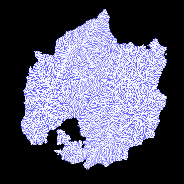
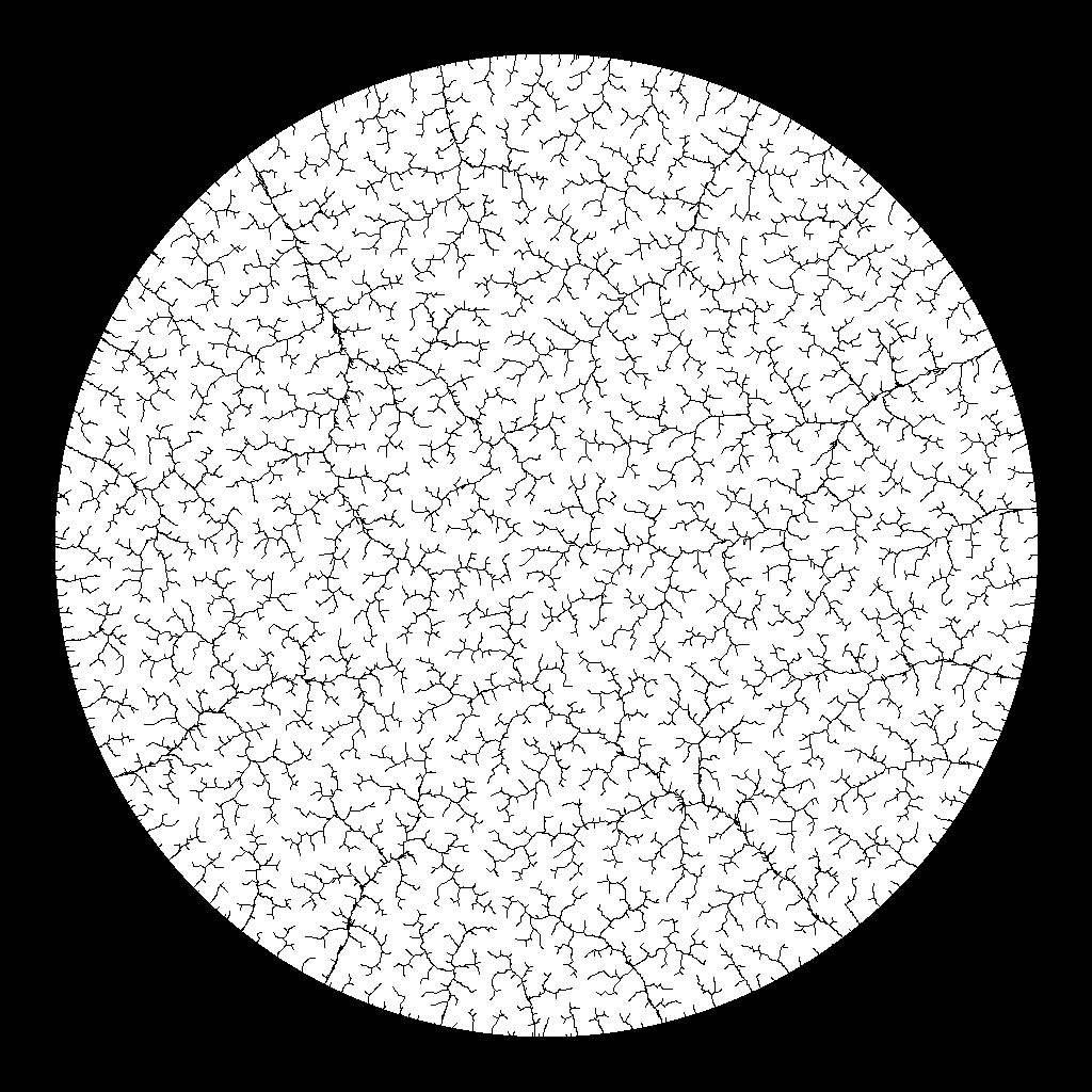
And so, in June of 2016, working out of a hacked-together Unity project, I finally managed to generate the following.

Of course, this wasn’t the first output I got from this technique; even from a cursory inspection, it should be obvious that this is a modified Brownian tree, not the basic implementation described and visualized above. I had hoped to include some of my very earliest results, but unfortunately I no longer have any samples of that. What’s shown above is the last result I achieved in my Unity prototype. This result proved the value of the project to me, whereupon I migrated the code to an ordinary .NET project that eventually became the Demiurge repository.
Since typing the above, I have scrolled back to the top of this post and added a “Part 1” to the title. I had originally intended to fit the entire discussion of the Brownian tree river generation technique into a single post; but considering how long this post is already, that might not have been my best idea. There will be a Part 2 (I probably won’t wait my usual two weeks between Demiurge posts to write it) which will discuss the details of the algorithm that generated the output above. In particular, I want to discuss what I learned from my initial implementation of the Brownian tree and what modifications I made to adapt it to my purposes: coarse-to-fine, cell-based point seeding, attachment sensitivity… In short, I’ll give a brief overview of all the ways in which the Demiurge implementation differs from a canonical, unmodified Brownian tree.
But this page is already too long, so that will have to be the topic of another post.
–Murray
