Not a river in a forest; a forest of rivers. That makes sense, right?
In this post, we’ll cover the first algorithm within Demiurge that can answer real questions about the map. How many major rivers are there? Which is the longest? What are the major watersheds? These and other similar questions all depend on a crucial piece of map information that is only one step — one complicated step — beyond the black-and-white river networks we’ve generated so far: the river forest.
What Is a River Forest?
Computer science concepts tend to have weird names. Names for new technologies are usually chosen because they “fit” in some readily appreciable way. Further study, however, will often lead to the discovery of additional related concepts. These will be given names conceptually related to the original name, even when the behavior of the newly-discovered concept has little to do with the real-world thing it’s being named after.
Trees might provide one of the best examples of this naming process gone wild. Trees in computer science are data structures that record hierarchical relationships among different data elements. The name “fits” in several ways: trees tend to have many branching paths, and in some ways they’re a generalization of the classic concept of a family tree. One step into the associated terms, however, and everything goes topsy-turvy: computer science trees grow downward, have a single root at the top, and consist entirely of branches and leaves without any sign of a trunk.
With all that said, a forest in computer science is defined as a collection of many trees. Anticlimactically straightforward, really.
So a tree is a data structure and a forest is a collection of trees. What, then, is a river forest? At this point, understanding a bit about the tree data structure is helpful (though beyond the scope of this post), but the short answer is that for our purposes in Demiurge we represent rivers as trees. I chose this representation because the hierarchical structure of river networks, where multiple smaller rivers can flow together to become one bigger one, is naturally represented as a tree, where multiple sub-trees can be grouped together under a single parent node. In particular, Demiurge represents rivers as trees of 2D locations, which can be most readily thought of as pixels.

Consider the image on the right, for example. Though it’s been scaled up, this image effectively contains 64 positions — 8 by 8 — that are either black or white. (White-ish; the “white” in this image has been changed to light gray to make the boundaries of the image distinguishable on a white web page.) If this appeared as a clipping from one of the Demiurge’s river network maps, the software would interpret this as a piece of land containing two rivers, one a tributary to the other. The way that decision is represented in data is as a tree.

To the left is the same image again, but marked up with position labels for the various pixels (and enlarged to make the labels readable [as much as possible, at least, given my handwriting]). It can now be readily seen that there are 13 locations marked as water amidst 51 marked as land, and that only one of the water locations is adjacent to the edge of the image. Rivers must always be flowing to the sea (according to Demiurge’s assumptions) and the sea clearly isn’t on this section of the map, so location (4, 0) is the only possible route by which the water at the other locations could flow out of this region. Demiurge would therefore treat (4, 0) as the root node of the river tree for this image. Again, the specifics of trees are outside the scope of this post, but the final river tree for this region would look something like the diagram shown below. (Note: the diagram only shows “interesting” nodes, which are the same ones given handwritten labels in the image to the left. This is an abbreviated form of the actual data structure, which contains a separate node for every location.)
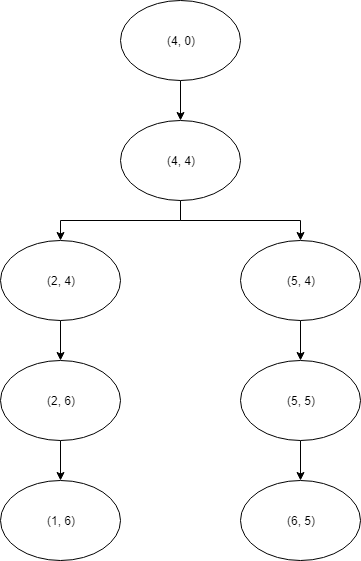
That is a river tree. If you had a bunch of those, you’d have a river forest. Thus, in order to fully understand the river systems we generated for in prior posts, we need to accumulate data like this for the whole map.
Trees and Tributaries
Though we touched on this briefly in the above section, I should call out specifically how tributaries are identified and treated by Demiurge. I’ve said many times that, according to Demiurge, all rivers must eventually reach the sea; this assumption is important for several of the algorithms I will describe. However, if you consider a river to be “a tract of moving water that bears a certain name,” the assumption about reaching the sea only rarely applies in the real world because most rivers — by name — are tributaries. The Missouri River, for example, is the longest river in North America; but instead of emptying into the sea, it empties into the Mississippi.
Tributaries as a concept are naturally handled by the trees that constitute the river forest. However, it’s important to realize that, because a single river tree contains the main river and all its tributaries, each tree in the river forest actually contains an entire drainage system. In short, there is not a one-to-one mapping between trees in the river forest and named rivers as they would appear on a map.
However, I did want the software to be able to answer questions about named rivers. (In fact, with only slight modification, it could be made to give names to all the rivers, though the results would be of questionable narrative value.) This is not difficult to do, but it requires making a decision at every location where two lesser rivers come together: which is the tributary and which is the main course? I investigated this problem for a lot longer than I should have, but in the end I never did figure out if there’s any pattern to how this decision has been made throughout human history. I suspect that most rivers were named and put on maps before the information about their tributaries was fully understood, causing the decision about which branch gets bear the name to be, in some cases, essentially random.
It wouldn’t be hard to make that decision random in Demiurge, too, and perhaps I should have done that. However, if only to be able to move on from the problem, I decided to use a simple hueristic to chose which of the two river branches was the main course: the longer one. That choice does mean that certain realistic situations — like the aforementioned case of the Missouri-Mississippi — cannot be achieved without modifying the algorithm; the longer river will always be classified as the main course. However, this simple hueristic provides the desired behavior the overwhelming majority of the time. It also makes questions like, “Which is the longest river?” very easy to ask and understand. And, if for some reason a user did want a different behavior, the hueristic wouldn’t be very hard to change.
The Hydrological Field: Finding Fresh Water
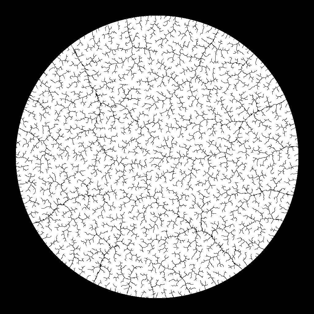
So now we come to the meat of the algorithm: actually building the river forest. At the end of the Brownian tree step, we were left with an availability field (philosophically identical to the black-and-white image shown above) that tells us which locations contain water and which contain only land. However, not every water location is part of a river, and the availability field has no way to distinguish between river and non-river (salt) water. To learn that information, we transform our availability field into a HydrologicalField.
The purpose of the hydrological field is simply to distinguish river locations from non-river locations. Essentially, this adds just one degree of granularity to the information already described by the availability field. Instead of the ” not water/water” answer the availability field could give, the hydrological field can distinguish “not water/saltwater/freshwater.” (For reasons that probably made sense to me at the time, I described these possibilities in an enum called LandType and respectively named them Land, Ocean, and Shore.) The algorithm for distinguishing between salt- and freshwater is one of those cases where I tried a dumb idea first, and it worked so well that I never needed to attempt something smarter.
To determine if a water location is freshwater, check the locations that surround it. If the ratio of land locations to water locations in the immediate vicinity is sufficiently high, that location is considered freshwater; otherwise, it’s saltwater. That’s it. No further intelligence is necessary, nothing fancier is useful. Just set a threshold and tune it. It works astonishingly well, which just goes to prove my personal engineering motto:
Never waste smart on something you can solve with stupid.
-Murray
Of course, this technique isn’t perfect — for this application, no technique would be — but I’ve yet to find a situation where a well-tuned hydrological map implemented this way gives wrong answers. Importantly, there’s little to no penalty for making the freshwater threshold overly permissive, so you can tune “on the safe side” and not worry that you’re going to degrade your results. The other artifact this can produce is that certain locations near the shore (which, logically, are probably saltwater) can sometimes be mislabeled as freshwater, especially if there’s a river mouth nearby. As an artifact, this isn’t necessarily wrong — these locations could represent a tiny freshwater creek, for example — but it’s also an easy artifact to detect and ignore at later stages.
There is, however, one major limitation of the hydrological map: it doesn’t understand lakes. It does recognize lakes, but it labels them as saltwater and treats them just like oceans. This is one aspect of a broader limitation of Demiurge where multiple systems, including the Brownian tree, don’t have the special-case behaviors necessary to deal with drawn-in lakes properly. This is, perhaps, the largest missing feature in Demiurge today. I thought about different ways to solve this problem, and it is solvable. However, I ultimately decided not to invest time in a solution because, for the map I cared about, I didn’t need a solution. There are two drawn-in lakes on my map, but both are essentially at sea level and didn’t need any special treatment. For now, then, just be aware that Demiurge currently treats all drawn-in lakes as salt lakes; the implications of this, and how it might be changed, will be discussed in future posts.
Contiguous Sets: Separating Drainage Systems
The hydrological map, once created, tells us every location which will appear in the river forest. Next, we need to group these locations into separate drainage systems. In other words, we want to split the set of all freshwater locations into many smaller sets, each of which contains all the locations for a single drainage system. Because all the locations of a single drainage system must be contiguous — i.e., there must be a way to “walk” from any location in the set to any other location in the set without “stepping” on anything outside the set — the utility library used for this operation is called ContiguousSets.
There are more than a few different functions in ContiguousSets, but the most important one for this conversation is the aptly-named FindContiguousSets. This function is generic, but it’s typically run directly against a hydrological field, which it then “organizes” into contiguous subsets bucketed by type. Note that this operation affects every location, not just freshwater locations. Consequently, the output of FindContiguousSets can be used to answer a broad variety of questions. How many river systems are there? How many bodies of non-river water are there? How many landmasses (islands, continents, etc.) are there? If you have a notion of scale — what is the distance in meters between adjacent pixel-defined locations — you can even approximate the size of every landmass, in square meters, just by studying the contiguous sets.
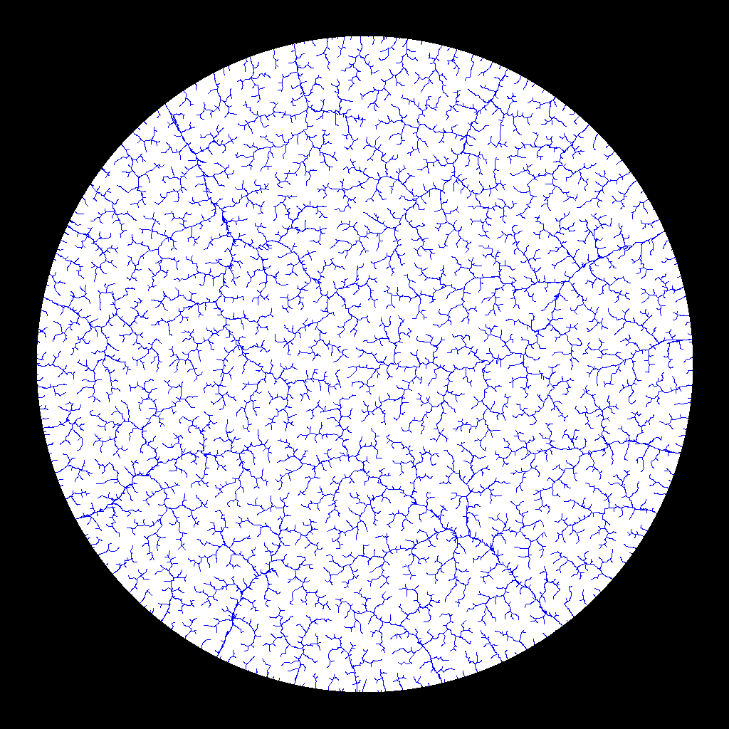
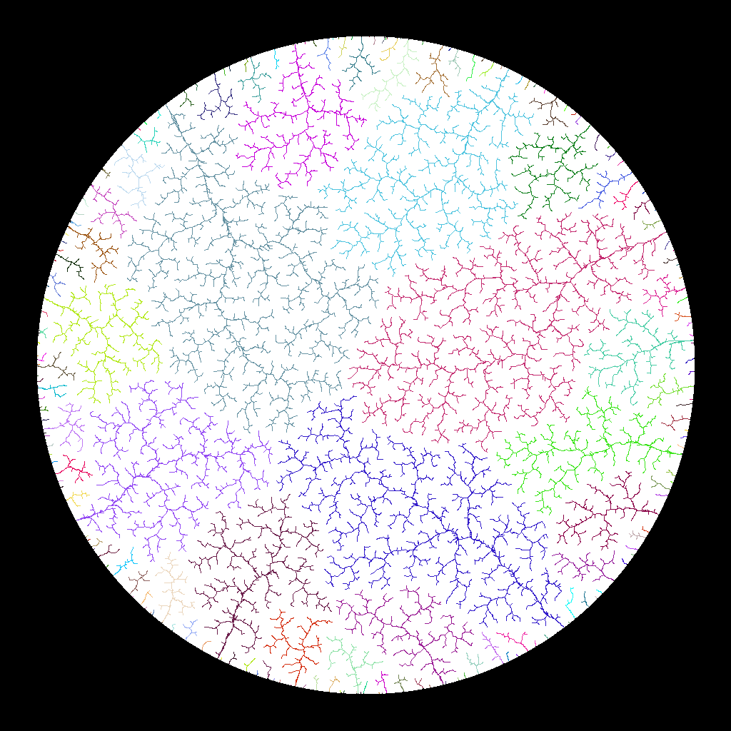
Typically, most maps will contain very few contiguous sets of “saltwater”: the sea and a small number of drawn-in lakes. Landmasses will usually be slightly more numerous, though that’s entirely dependent on the original “coastline” map drawn by the user. Freshwater sets, however, are often very numerous. The map below, for example, contains 197 contiguous sets of freshwater locations. Each of these sets represents a separate drainage system — a separate tree in the river forest.
Creating the River Forest
This brings us at last to the river forest itself. Armed with the contiguous sets, all we have left to do is to turn those sets of locations into properly-structured river trees whose roots are adjacent to the sea.
But before we discuss that, I should call attention to a very important assumption upon which this step depends. Demiurge assumes that the contiguous set of locations which constitutes a river only touches saltwater at a single location; in other words, rivers only have one mouth. This, as with the lakes, is a case where the assumption does not entirely match reality, but it applies in such an overwhelming majority of cases that the simplification was worth it. Very few real rivers have two mouths, and none of the rivers in the map I was working on did. Again, as with the lakes, there are ways to change the software to support things like multiple mouths and rivers traveling from drawn-in lakes to the sea (which is not currently supported, but also cannot be generated by Demiurge at present due to the nature of Brownian trees). Those features simply haven’t been necessary for my use cases so far, so the work has remained purely theoretical.
So, assuming a contiguous set only encounters the sea at a single location (the implementation is robust to their being several freshwater locations together at the mouth of a river, it’ll just choose one at random), the task of turning a contiguous set into a river tree is extremely simple. All we have to do is find the root pixel (again, if there are several good candidates close together, pick one at random), then use a standard breadth-first traversal to add the rest of the locations in the contiguous set to the tree in the order they’re encountered. And that’s exactly what the code does. The river tree generated by this algorithm can tell us all manner of things about the drainage system it represents: maximum length, number of tributaries, approximate drainage area, and even rough flow volume estimates. All that from one river tree. Once we do the same for every drainage system — once we have, at long last, the river forest — we can learn a ton of details about the entire map.

This map contains one ocean, one major landmass, and 708 different rivers sufficiently large to merit names. Assuming each pixel represents one square kilometer of terrain, this map displays 381,643 square kilometers of ocean, 612,386 square kilometers of dry land, and 54,547 square kilometers of land containing rivers. The total continental area of the landmass is 666,733 square kilometers — about 10% smaller than Borneo, and almost 200% larger than Great Britain. Of the 708 noteworthy rivers, 136 are main course rivers that empty into the ocean; the remaining 572 are tributaries. The longest main course river is 529 kilometers long, the shortest is 5 kilometers, the average is 54 kilometers, and the median is 22. The largest river system includes 8,605 kilometers of waterway, but drainage system size drops off quickly: only twelve drainage systems contain more than 1,000 kilometers, and the median is a paltry 33. 249 tributaries empty directly into the main course of their river system, while the remaining 323 are tributaries of tributaries. The largest river system on this island is about 30% larger than the Thames by length, and 93% smaller than the Nile.
Perhaps details like that are boring; I certainly wouldn’t recommend sticking them directly into a narrative. However, they do give context to the world in a manner unlike anything I’ve encountered from any other tool. These are the sorts of details that readers needn’t perceive directly, but that characters may need to know in order to make sensible decisions. And there’s more information that could be gleaned from what’s above. You could estimate flow volume to make predictions about navigability. From this, you could begin to explore likely routes of trade — places where barges can go, places where portage or caravans can overcome small obstacles, and places rendered remote and nigh inaccessible by the shallowness of their waterways. You can establish the borders of a kingdom along waterways or watersheds, count the productive valleys within those borders; you can estimate the size of the government you’d need to oversee those valleys, the kind of infrastructure you’d need to transport taxes, and even the expected size and composition of a kingdom’s annual yield. Some of those questions I have yet to explore at all, and my approach to them remains purely theoretical. Others, however — borders and trade routes in particular — I have explored more deeply; I hope you’re as excited as I am to discuss those in future posts.
As a final note, you may have noticed that the “tributary map” visualization in the image above actually contains significantly more information than can be gathered from the river forest alone. For one thing, that visualization shows drainage basins as well as waterways; for another, tiny rivulets of an insufficient length have been excluded from both the visualization and the factoid litany following it. (This is the reason there were 197 contiguous sets of freshwater, but only 136 main course river systems worthy of note.) This happened because, for my own convenience in writing this blog post, I chose to use an existing visualization I had created to represent a WaterTableField. Water table fields are the next step in the Demiurge algorithm; they build upon the river forest and allow us to answer even more questions about the topography of the world represented by our map.
But I’ve already crammed too much into this document, so that must be the topic of another post.
–Murray
