This is going to be, by far, the most technical and least prosaic post I’ve yet written for this site. Following up on the overview of Brownian trees I presented in Part 1, this post will be dedicated to enumerating and explaining the modified Brownian tree used in Demiurge. In other words, we will be looking at code. To create the river network generator for Demiurge, I made several modifications to the basic Brownian tree concept, but only three are really worth talking about: coarse-to-fine, cellular seeding, and halting conditions.
Foreword: Fields
Fields, in the context of the Demiurge codebase, are not a concept specific to the Brownian tree or any other single part of the Demiurge pipeline. However, because they are important and this is the first time we’ve encountered them, I’ll take this opportunity to explain.
A field, in Demiurge terminology, is simply a data structure in which data values are stored in spatial relationship to each other, usually in 2D. Fields are the fundamental data container with which different parts of the Demiurge pipeline communicate with each other. Most operations take one or more fields (among other data) as input and produce fields as output. The simplest form of a field is just a multidimensional array, and in fact the most common implementation of a field is exactly that. More sophisticated fields allow for non-integral addressing, sparse data, and even lazily-evaluated transformations — but that’s a lot more power than we need right now.
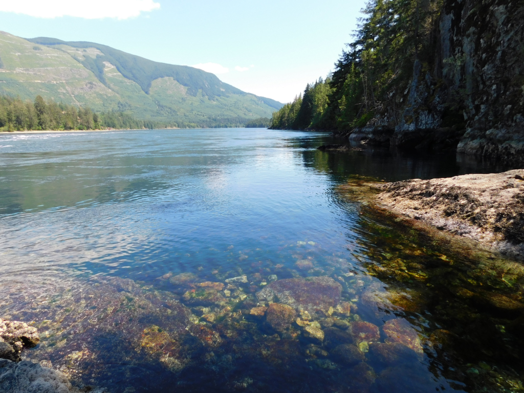
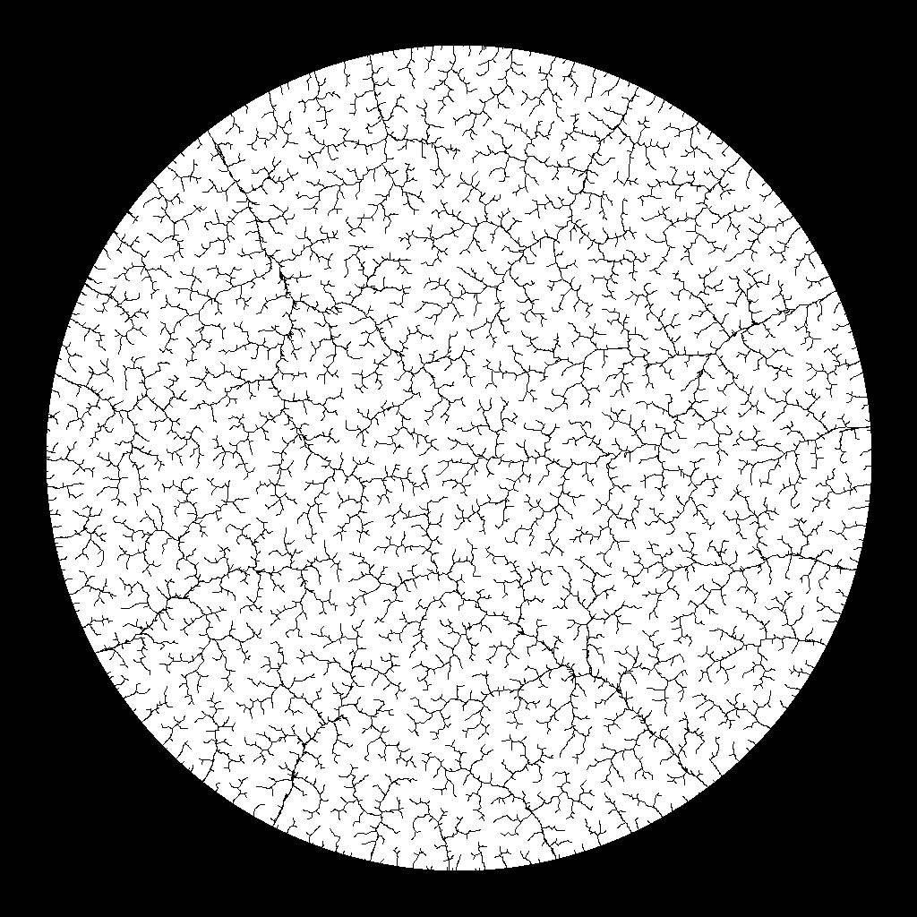
Brownian trees in Demiurge only deal with Field2D<BrownianTree.Availability>, which you can think of simply as a black-and-white image. The Brownian tree’s input field is a direct interpretation of the very first input map provided to the Demiurge system, interpreting black pixels (representing water) as Unavailable and white pixels (representing probable land) as Available. From this input, the Brownian tree would build its river system out into the Available pixels, eventually producing another field of availability that can be interpreted as water and land. In short, using availability fields as interpretations of black-and-white images, the Brownian tree takes something like the image on the left and turns it into something like the one on the right.
Lest it cause confusion, I should also mention the third possible value of the Availability enum: Illegal. This value was introduced as part of an experiment to enable the manual designation of watersheds by specifying locations where water could not go. I’ll briefly discuss this experiment later in this post. However, though I believe the idea worked reasonably well, it didn’t turn out to be very useful for my scenario; the overwhelming majority of my river networks have been generated from Available and Unavailable locations alone.
Coarse-to-Fine
The earliest version of my river network generators were very literal interpretations of the classic Brownian tree described in Part 1. To put it mildly, these generators were slow. Particles were simulated as pixels, so each iteration of the algorithm would put a single particle at a random Available location, then move that particle around (in one-pixel steps) until it came into contact with an Unavailable location. That works reasonably well if the probability of encountering an Unavailable location is relatively high; but if the particle was dropped in, say, the middle of the gigantic white circle show above, that particle could travel for an unbearably long time before its Brownian motion took it near to an Unavailable location.
Note that this behavior was primarily related to image resolution, which in a pixel-based implementation of Brownian motion is tantamount to step size. Smaller images could be processed faster because particles wouldn’t need to travel as far before they were allowed to stop, even in the worst cases. This observation inspired me to use an approach that I describe as coarse-to-fine, but which might be more familiar as a variation on iterative refinement.
The basic idea was that, instead of particles taking 1-pixel steps regardless of the state of the map, they should be allowed to take large steps in early iterations (where the probability of encountering an Unavailable location is expected to be low), and step size should be decreased as the map becomes more densely populated with Unavailable locations. In essence, this algorithm treats early iterations on a high-resolution map as though they were being conducted at a lower resolution, enabling larger steps and allowing Unavailable locations to be “encountered” from further away.
The implementation for this technique begins on line 43, where the step size is initialized to a ludicrously large value. This doesn’t matter, however, as over-large step sizes will quickly be reduced to reasonable values. This initialization is immediately followed by the core loop of the coarse-to-fine implementation, which runs passes of the algorithm at diminishing step sizes until a terminating condition is met. We’ll revisit that loop in the following two sections; for now, it’s only important to note that stepSize is halved whenever impact — a value which represents how much change an iteration resulted in — is below a certain (unfortunately hard-coded) threshold.
There is one more block of code I want to call attention to in this section: lines 90 through 96. This complicated-looking loop (I apologize profusely for packing as much garbage as I did into line 91 — I didn’t fully appreciate code readability as a goal in those days) does little more than draw a “line of unavailability” from the place where the particle stopped to the Unavailable location it encountered. However, it makes use of a variable we haven’t seen before called maxSegment, which you can see from line 47 is actually hard-coded to 5, regardless of step size. This technique was introduced to mitigate an unintended consequence of the coarse-to-fine approach. When a particle is allowed to take large steps and “encounter” Unavailable locations from far away, connecting that particle to the larger corpus of Unavailable locations (without which a “tree” cannot be formed) is most readily done by drawing a “line of unavailability” from the particle to the location it encountered. However, when step sizes are very large, this results in obvious, unnatural-looking straight lines that detract from the output’s plausibility as a river system. To counter this, maxSegment puts a hard cap on the length of the “line of unavailability”; instead, a small segment is drawn from the encountered Unavailable location toward the encountering particle’s location, thereby maintaining the Unavailable tree’s coherency without drawing straight lines beyond a predefined acceptable length. Using this technique reduces the rate at which coarse iterations populate the map with Unavailable locations, thus requiring more iterations to “fill in” the map. However, the technique allows larger-than-ever step sizes to be used without compromising the quality of the output, which balances out the need for additional iterations by making iterations overall less expensive.
Also, a final note on directional artifacts. If you look back at the Brownian tree video I linked to in Part 1, you may notice subtle directional artifacts in the results: the tree tends very slightly to develop vertically, horizontally, or at orderly diagonals. This artifact is a consequence of representing particles as pixels, which live a rectangular world and (given their own preferences) move in rectangular ways. The details of this phenomenon are beyond the scope of this discussion (and beyond my expertise), but having a rectangle-based “encounter” mechanism produces subtle but visible artifacts in the resulting Brownian trees. These artifacts existed in my earliest implementations, but they disappeared when I began using a coarse-to-fine approach. This may seem counter-intuitive because, even in the current implementation, movement is still rectangular, caring only about Manhattan distance. However, movement itself isn’t what actually produces this artifact; what matters is collision, or the “encounter” mechanism, and that comparison is based on Euclidean distance.
Cellular Particle Spawning
Once the raw execution time had been brought down to an acceptable level, a new problem began to emerge: density. It is the nature of rivers (at least, according to the assumptions of Demiurge) that they’re everywhere: if rain falls on a patch of ground, there must be a river nearby by which the water can depart. My early Brownian trees, however, had a tendency to “fence off” certain areas and neglect to generate rivers there. Once a region is relatively isolated by Unavailable locations, then the only way for the Brownian tree to grow into that region is if new particles are spawned there, because particles spawned elsewhere will find it difficult or impossible to “wander” into the isolated region. The smaller such a region is, the less probable that a particle will be spawned there by a truly random sampling. Waiting for improbable events means enduring many iterations; thus, as I strove for consistent distributions of waterways, my execution time rose again.
I admit that I thought about this problem — that random particle spawning wasn’t putting particles where I wanted them — for an embarrassingly long time before I came up with the obvious solution: don’t spawn particles randomly. Because I knew I wanted particles throughout the map, I decided to try dividing the map into localized cells, each of which would have a particle spawned at a random location inside the cell. This idea worked very naturally with the coarse-to-fine approach, and with the two ideas together I was able to formalize my notion of a pass.
A “Brownian tree pass,” in Demiurge terminology, is a procedure run over an availability field which very slightly grows a Brownian tree in that field. One pass corresponds to a single execution of the aptly-named AddBrownianTreePass method, defined on line 53. The cellular spawning behavior in particular is defined on lines 56 through 62. Apparently it uses step size as cell size, instead of defining that as a related but separate concept. (Trust me, I’m as surprised as you are; it can sometimes be truly depressing to read your own years-old code.)
The essence of the procedure is extremely simple: spawn a new particle in every cell on the map, then process each spawned particle in turn as the next particle of the Brownian tree. There are, however, two nuances I want to call attention to, the first of which is the behavior on lines 69 through 71. These lines cause the spawned particles to be processed in random order, which is a surprisingly important part of the algorithm. Note that the spawning code above operates by iterating through i and j, left to right and top to bottom. Consider what would happen if we added those particles to the Brownian tree in that same order. As the tree evolved, it would consistently be one generation “older” above and to the left during the execution of a pass. “Older” means “more densely populated with Unavailable locations,” which means that, in the general case, there would tend to be more things for new particles to “encounter” up and to the left than down and to the right. This ordering problem introduces a directional bias into the river generation which results in surprisingly obvious visual artifacts as rivers noticeably tend to flow more north and west than east and south (assuming conventional North American map orientation relative to the compass). Processing the particles in random order eliminates these artifacts by causing the tree to be “older” in unpredictable locations, preventing any directional bias from forming.
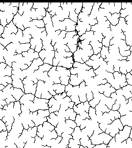
The second nuance I want to call attention to is the concept of impact. Philosophically, impact represents how much was accomplished by a given Brownian tree pass; this is measured, as can be seen on line 98, by counting the number of cells which resulted in the Brownian tree being actually grown. You see, not all particles eventually grow the tree because, in two different circumstances, particles can be discarded without having accomplished anything. The first — and by far the more common — of these conditions is if a particle is spawned so close to existing Unavailable locations that it “encounters” something without even having to move. This condition was introduced because, without it, the algorithm continues to add little rivers and branches to areas that are already thoroughly drained, creating a characteristic “tangle” artifact that detracts from the tree’s representation of a river (see the image below for an example). The second –and much less common — way for a particle to be discarded is for that particle to move to an “illegal” location. This usually means that the particle has somehow wandered off the edge of the map, but it can also happen if a particle gets too close to an Illegal location as described in the Availability enum. Without going into too much detail, this was the mechanism by which watershed designation is implemented: specify a line (or region) of Illegal locations, and rivers will never cross it because particles that get too close will simply be discarded.
Returning to the notion of impact, the idea that particles can “fail” to change anything leads naturally to the utility of measuring a “success rate” for particles in a given pass. This, in turn, leads naturally to the final Brownian tree modification I want to discuss.
Halt Conditions
This was always a question with Brownian trees: how do I know when to stop? Early on, I ignored the problem, simply hard-coding iteration counts and changing the number if the result didn’t look the way I wanted. However, that approach could only go on for so long, and I knew I would eventually need to find a way to automatically determine a good stopping point for my river generation algorithm. Fortunately, once I’d introduced the coarse-to-fine and cellular spawning modifications to my algorithm, the concept of impact gave a very easy answer to the question of when to stop: stop when it’s no longer useful to continue.
Note that this isn’t just a question of when to halt generation on the entire Brownian tree, though that is part of it. This actually circles back to line 49, which determines when to modify stepSize and progress from a coarser set of passes to a finer set. With all of these concepts in place, we can finally present a full representation of the Demiurge Brownian tree algorithm.
- Initialize stepSize to a large number.
- Execute a single Brownian tree pass with stepSize and record the impact.
- If impact was above a certain threshold, return to step 2 of this procedure.
- If impact was below a certain threshold, divide stepSize by 2.
- If stepSize is larger than minimumSensitivity (given as a parameter, name is related to other variables not discussed here), return to step 2 of this procedure.
- Otherwise, halt the algorithm and declare the Brownian tree to be complete.
Note that these halting conditions do not make guarantees about the output, but they do make it highly probable that the final Brownian tree will be fairly uniformly populated with Unavailable locations to an approximate density determined by the minimumSensitivity parameter. If minimumSensitivity is a small value, then the algorithm will continue until the tree is densely populated, leaving little space between disjoint Unavailable locations; if minimumSensitivity is large, more space will be left such that the resulting map will appear more “spider-webbed.” There is, however, one guarantee that the Brownian tree explicitly provides: no two disjoint “strands” of Unavailable locations will ever actually touch each other. This guarantee is enforced by having the “encounter” mechanism choose only the nearest point of attachment, thus preventing two disjoint strands from ever “growing over” each other. Keep this guarantee in mind; it will be important when we transform our Brownian tree, with its strands of Unavailable locations, into a hydrological field that we’ll use to discover and describe the complete river system of our map.
But that will be the subject of another post.
–Murray
P.S.
Looking at some of this old code today, I was a little surprised. Mismatched names, confusing loop conditions, unnecessary allocations all over the place… Hmm. In fairness, this code was never intended to be “production quality”; I built this only for myself, coding in the fragmented hours between working as a software engineer and writing as an aspiring novelist. Nevertheless, I do want to make it abundantly clear that neither BrownianTree.cs nor any other code in Demiurge should be taken as an example of high-quality C# or careful engineering. Bear in mind the circumstances under which this library was written, and please try to forgive the brazen hacking of a younger Murray who wrote this while tired after work, unsure of where the project was going, and possibly on the adventurous side of the Ballmer peak when at least some of this code was written.
But hey… I mean, it works, right? –M